Required packages for this vignette

Run this to install the necessary packages for visualization and data processing

install.packages("cowplot") # for making the grid plot
install.packages("BiocManager")
BiocManager::install("SingleCellExperiment") # for using the SingleCellExperiment data format
install.packages("forcats") # for working with categorical data

library(corgi)
library(ggplot2)
library(cowplot)

Download data

Download data from the Hemberg lab website

yan <- readRDS(url("https://scrnaseq-public-datasets.s3.amazonaws.com/scater-objects/yan.rds"))
deng <- readRDS(url("https://scrnaseq-public-datasets.s3.amazonaws.com/scater-objects/deng-reads.rds"))

Preprocess data

rownames(yan) <- toupper(rownames(yan))
rownames(deng) <- toupper(rownames(deng))
shared_genes <- intersect(rownames(yan), rownames(deng))

# Get rid of the spike-in genes

shared_genes <- shared_genes[-grep("ERCC", shared_genes)]
yan <- yan[shared_genes, ]
deng <- deng[shared_genes, ]

Run CORGI

Warning: the figure displayed below used results that ran for 3 hours. For this vignette, we set the run time to 10 minutes, which should give reasonable looking results. To get a closer to the figure shown below change run_time = 10*60 to run_time = 3*60*60

corgi(
  normcounts(yan),
  counts(deng),
  run_time = 10*60
) -> corgi_output

Select the genes

corgi_gene_set <- corgi_select_genes(corgi_output, 100)

Combine the datasets

combined <- 
  combine_sces(
    sce_list = list(Yan = yan, Deng = deng),
    levels = c("zygote", "2cell", "4cell", "8cell", "16cell", "blast")
  )
cell_type <- combined$cell_type
batch <- combined$batch

Perform dimensionality reduction

mds_all_genes <- spearman_rho_mds(counts(combined))
mds_corgi <- spearman_rho_mds(counts(combined)[corgi_gene_set, ])

Plotting

my_color_palette <- c("#000000", "#E69F00", "#56B4E9", "#009E73", "#F0E442", "#0072B2", "#D55E00", "#CC79A7")
my_shape_palette <- c(16,1)
qplot <- function(...){
  ggplot2::qplot(...) +
    scale_color_manual(values = my_color_palette) +
    scale_shape_manual(values = my_shape_palette)
}

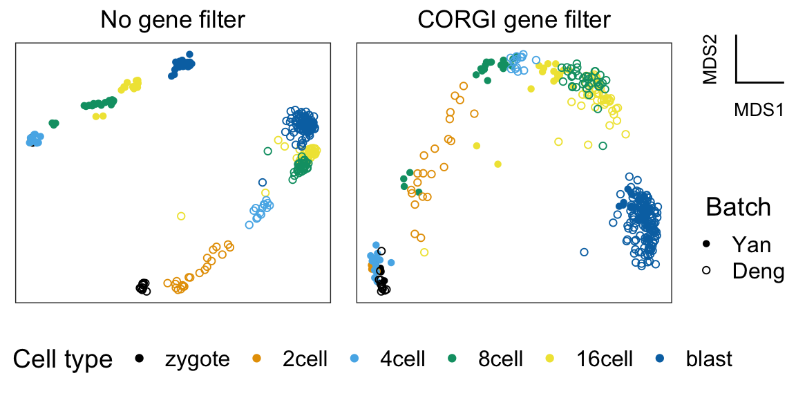
plt_all <- plot_dimensionality_reduction(mds_all_genes, batch, cell_type)+
  ggtitle("No gene filter")
plt_corgi <- plot_dimensionality_reduction(mds_corgi, batch, cell_type)+
  ggtitle("CORGI gene filter")


color_legend <- get_color_legend(cell_type, my_color_palette, legend.position = "bottom",ncol = 6)
batch_legend <- get_shape_legend(batch, my_shape_palette)
axes_legend <- get_axes_legend("MDS")

plot_grid(
  plot_grid(
    plt_all,
    plt_corgi,
    plot_grid(axes_legend, batch_legend, nrow = 2), 
    nrow = 1,
    rel_widths = c(3, 3, 1)
  ),
  color_legend,
  nrow = 2,
  rel_heights = c(4,1)
)

Get started: Pre-implantation embryo development in human and mouse

Yutong Wang

2019-10-24